Here I have implemented a customer lifetime value prediction model to calculate how valuable a customer may be for an e-commerce store called CDNow (Currently not in service). But first, what is customer lifetime value? Customer lifetime value is the total worth of a customer to a business or company over the entire period of their relationship.
Why is this metric calculated?
- Knowing the CLV helps businesses develop strategies to acquire new customers and retain existing ones while maintaining profit margins.
When I started my Data Science internship at 42hertz INC, this was one of the first projects that I worked on. Let me tell you a little about it:
The dataset that I got from CDNow was fairly simple. It contained useful information such as customer id, customer index, date, quantity and amount. One of the easiest ways of implementing a CLV prediction model according to me is using the lifetimes library in Python which may not be known by many. Python really has it all!
One of the ways to calculate the CLV is by using the Pareto/NBD model which is what I implemented. The Pareto/NBD model uses order history as the primary input, and in particular takes into account the frequency and the recency of orders by calculating the Recency-Frequency-Monetary Value matrix (Or RFM matrix). We need these numbers calculated separately for every customer in the cohort. These are:
-
Recency — The time between the first and the last transaction
-
Frequency — The number of purchases beyond the initial one
-
T — The time between the first purchase and the end of the calibration period
-
Monetary Value — The monetary/proportional value of a customer when compared to the rest of the cohort
The lifetimes library does a great job of wrapping the model’s equations into handy functions.
from lifetimes.utils import summary_data_from_transaction_data
rfm = summary_data_from_transaction_data(cdnow_transactions, 'customer_id', 'date', observation_period_end='1997-09-30')
This gives the Recency, Frequency and T values.
Now, the model is fit.
from lifetimes import ParetoNBDFitter

pnbd = ParetoNBDFitter()
pnbd.fit(rfm['frequency'], rfm['recency'], rfm['T'])
With the model and the R,F,T values, we can find other useful information about the data and the customers, such as:
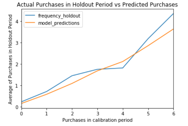
Here is a plot showing the actual purchases in holdout period versus the predicted purchases:
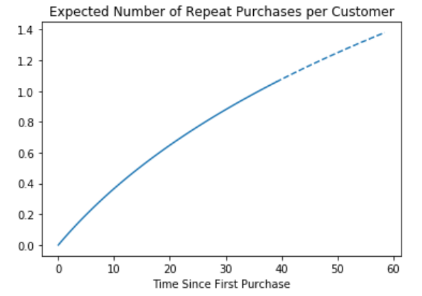
Here is another plot showing the expected number of repeat purchases per customer:
Now, the idea was to predict customer churn, so we are not interested in the probability of being alive, but the opposite of it:
1 - pnbd.conditional_probability_alive(rfm['frequency'], rfm['recency'], rfm['T'])
And there you have it! You now know some valuable information about your customer.
There are many more functions in the lifetimes library that you can play around with to find more insights about your customer.
If you are interested in reading more about the Pareto/NBD model or its other alternatives, you can read this paper: Peter S. Fader
You can find the code here: GitHub
Thanks for reading!